

Issue 06 · 3 September 2026 · Addendum added the same day · 941 trades · 13.6 years
We spent a week taking other people's backtests apart. Then we pointed the same method at the strategy running live in our own account, and found exactly the flaw we had been criticising in everyone else.
Real in sample · Fails out of sample · Verdict, revised: does not beat the index
t = 3.27 in sample · t = 1.60 out of sample · addendum: no threshold from 50 to 150 beats buy-and-hold out of sample
01 / WHY THIS ONE IS DIFFERENT
This is the strategy we have money on
Every other issue has examined somebody else's work. This one examines ours. The Saty Phase Oscillator is the strategy running in our live paper-trading account right now — one Nasdaq contract, an entry window between 09:40 and 11:00 New York time, flat by the close. It is the reason the lane exists.
A reader asked a simple question that we had never asked of it: is it more profitable than just buying the index? We had asked that of Connors RSI(2) a day earlier and the answer reversed our verdict. We had never turned it on ourselves.
Across the full history the answer looked good. 941 trades since January 2013, 55.3% of them winners, and at the account level — capital in one-month Treasury bills when flat, buying the index when the signal fires — it returns 6.84% a year at 6.2% volatility with a worst drawdown of 11.3%. Buying and holding the Nasdaq 100 over the same period returns 15.07% at 18.8% volatility and draws down 35.6%.
Less money, much less risk. A Sharpe ratio of 0.81 against the index's 0.75. We nearly published that.
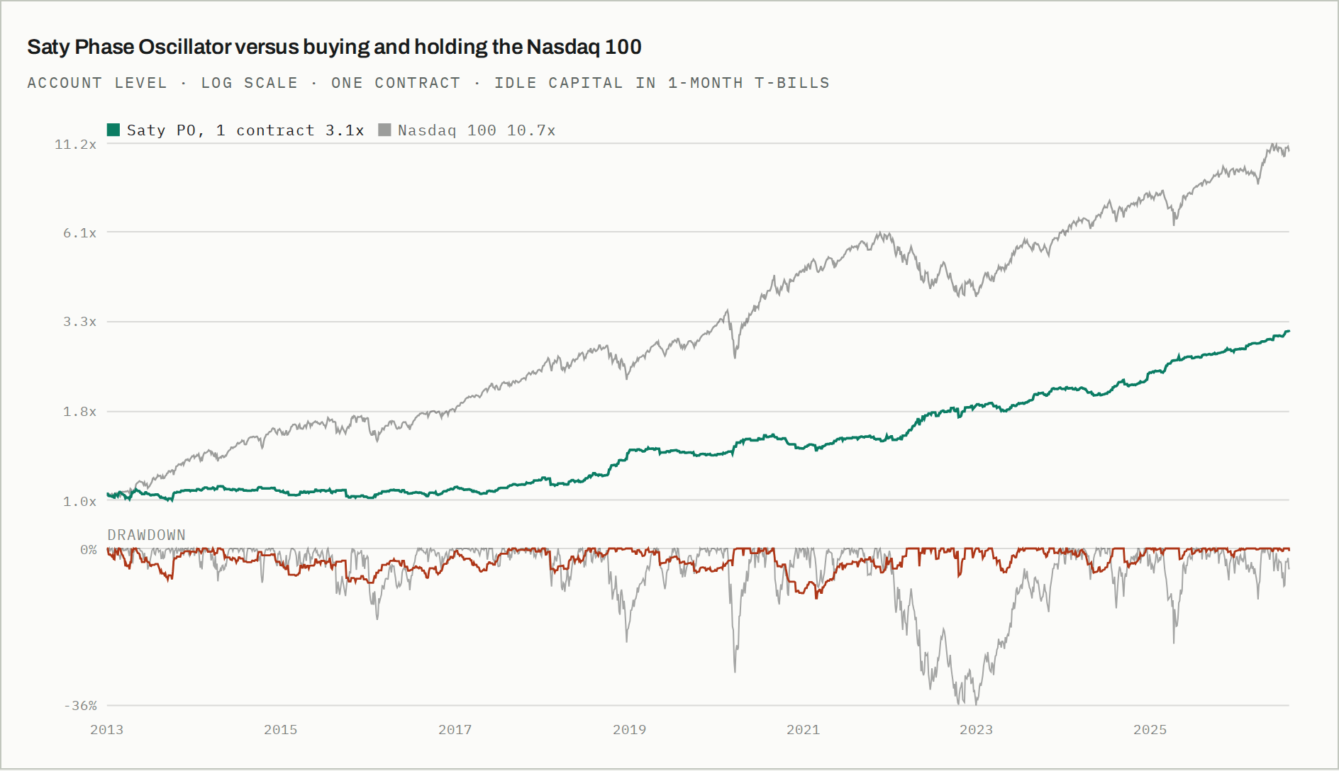
Growth of one unit of capital, with the drawdown of each series below. The strategy is in the market on 22% of sessions and in cash the rest of the time, which is what produces the shallow drawdown profile and the shortfall in total return. Both series are gross of tax.
02 / THE SPLIT
Then we cut it in half
The strategy was developed on data from December 2018 onward. Everything before that — January 2013 to November 2018 — is data it never saw. That is a genuine out-of-sample window, and it is the first thing we check on anyone else's work.
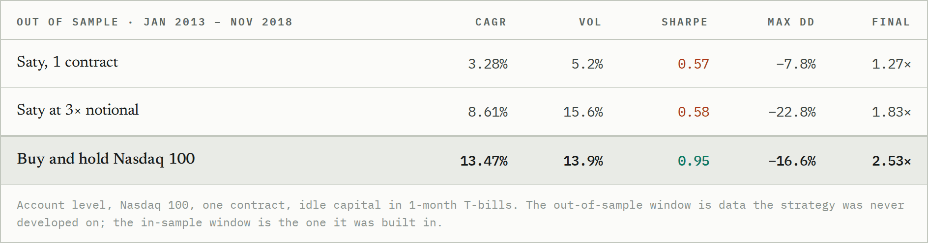
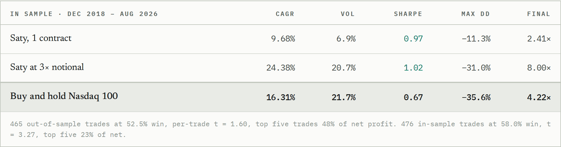
The average trade is three times larger in the window the strategy was built in. +0.145% against +0.048%.
Win rate 58.0% in sample against 52.5% out. Per-trade t-statistic 3.27 against 1.60, which is not significant at any conventional threshold. Out of sample the top five trades account for 48% of all profit — the same concentration that failed the opening range breakout in our first batch.
And the direction of the comparison flips. In sample, Saty beats the index on Sharpe by a wide margin, 0.97 to 0.67. Out of sample it loses, 0.57 to 0.95. The full-history figure that looked like a win is the average of a strong half and a weak half.
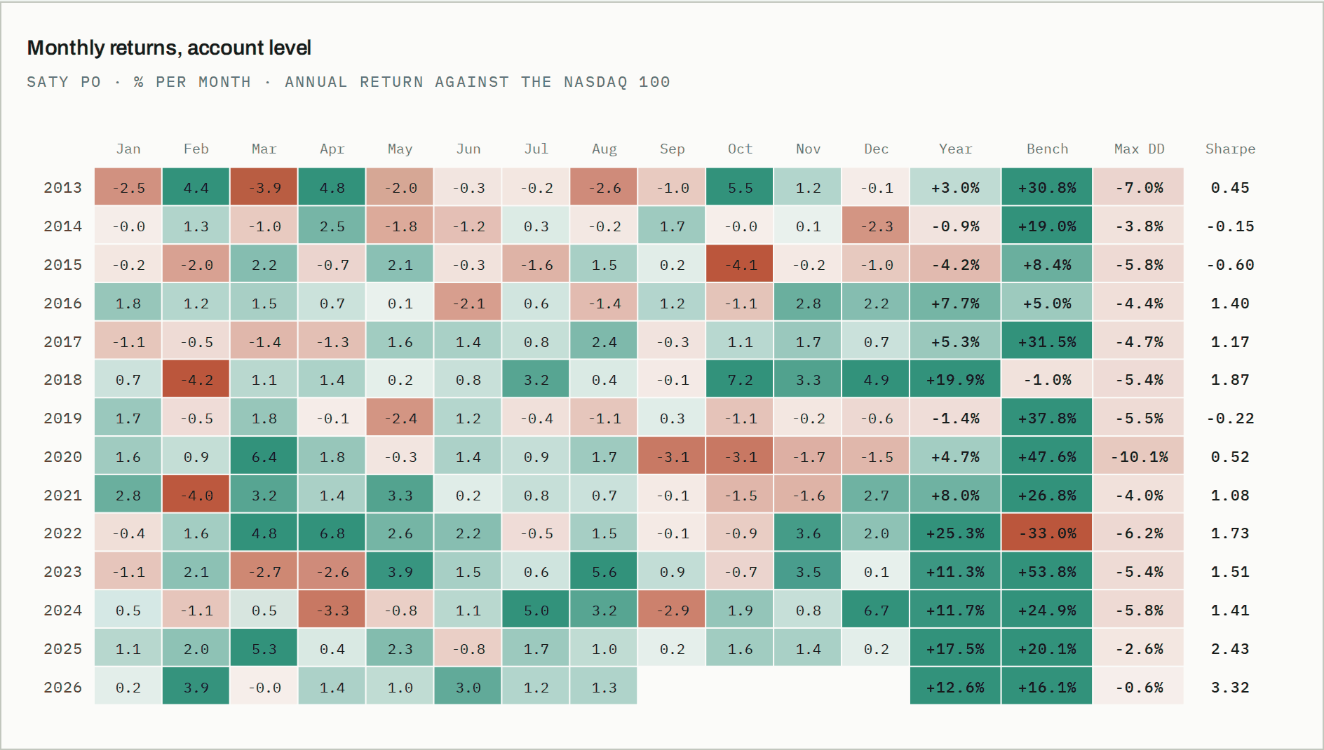
Green is a positive month, red negative, intensity scaled to magnitude. The Bench column is the Nasdaq 100 over the same year. The pre-2019 rows are the out-of-sample period: consistently positive, consistently small, and consistently behind an index that was compounding at 13% a year with a 0.95 Sharpe.
03 / THE COUNTER-ARGUMENT
The case that this is regime, not overfitting
We want to put this as strongly as the finding, because we think it is genuinely unresolved and because we would demand the same fairness if we were the ones being examined.
2013 to 2018 was an extraordinarily smooth Nasdaq melt-up. Buying and holding posted a 0.95 Sharpe ratio over those six years, which is an exceptional number for an equity index and a brutal benchmark for anything defensive. 2018 to 2026 contained the COVID crash and the 2022 bear market, and buy-and-hold's Sharpe fell to 0.67 while Saty's shallow-drawdown profile did exactly what it is designed to do.
A defensive intraday strategy should look bad against a melt-up and good against a decade with two crashes in it. That pattern is what you would expect from a real strategy running through different weather, and it is also what you would expect from an overfitted one. The two explanations predict the same data.
465 out-of-sample trades at a t-statistic of 1.60 cannot separate them. That is the honest state of knowledge, and anyone who tells you they can resolve it from this sample is selling something.
Update, same day: the split alone cannot separate them. The parameter neighbourhood can, and it does — see the addendum that follows.
ADDENDUM · SAME DAY
The test we said we could not run
A few hours after publishing, we found the test. Section 03 says 465 out-of-sample trades cannot separate regime from overfitting, and that is true of the split on its own. The parameter neighbourhood can, and we owe it to you to show it.
The strategy enters when its oscillator crosses ±100. We re-ran it at every threshold from 50 to 150 in steps of ten, in both windows, at the account level, against the same buy-and-hold benchmark. The logic is simple. If the in-sample advantage were regime, every threshold should show it. If it were parameter selection, 100 should sit on a peak that the out-of-sample window does not share.
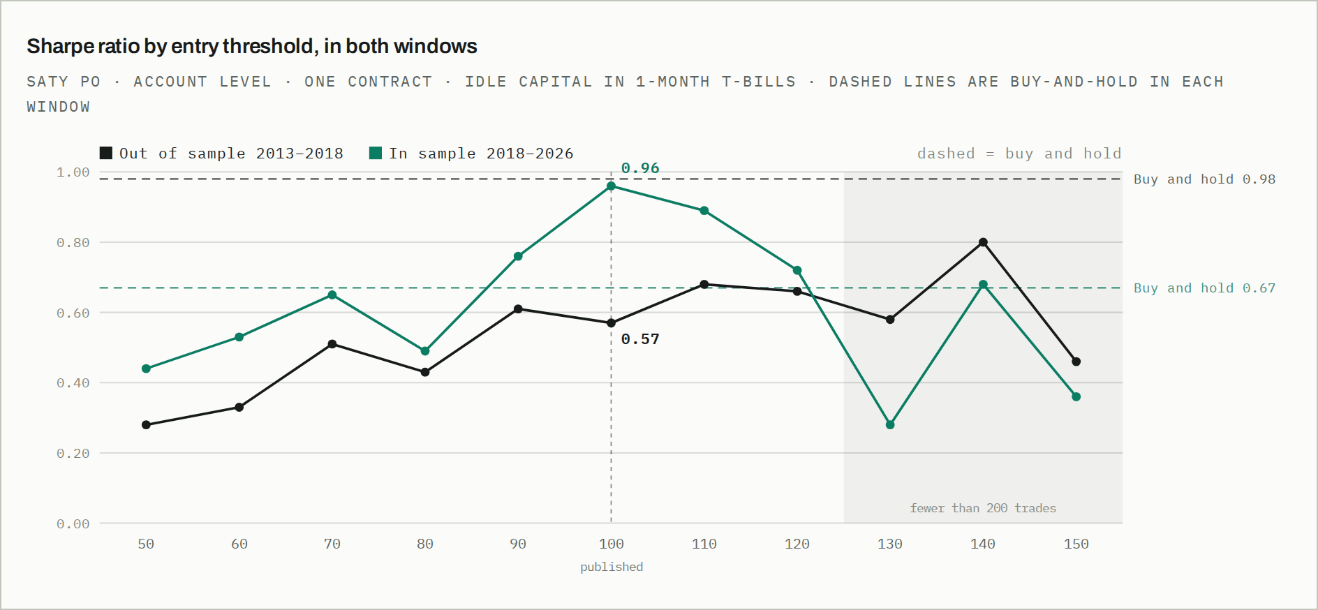
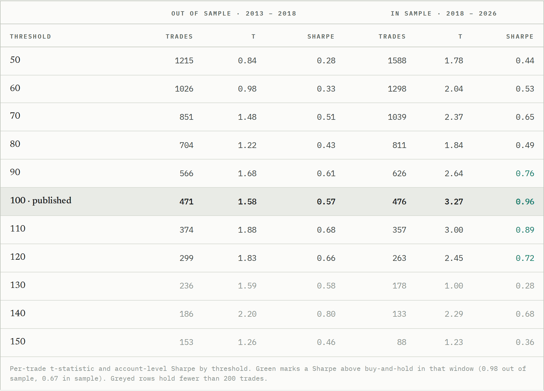
Fixed calendar windows: 2013-01 to 2018-11 and 2018-12 to 2026-08. Cells at 130 to 150 hold fewer than 200 trades each and are too thin to read on their own. Buy-and-hold reads 0.98 here and 0.95 in section 02 because the fixed window counts the first session of 2013, a +3.1% day; the strategy's own figures are identical in both.
In sample, 100 is the peak of a hump that runs from 90 to 120: 0.49 at 80, 0.76 at 90, 0.96 at 100, 0.89 at 110, 0.72 at 120. The published figure is the best of the eleven thresholds we tested. Out of sample there is no peak at 100. The curve drifts upward to 140 and no threshold reaches buy-and-hold's 0.98.
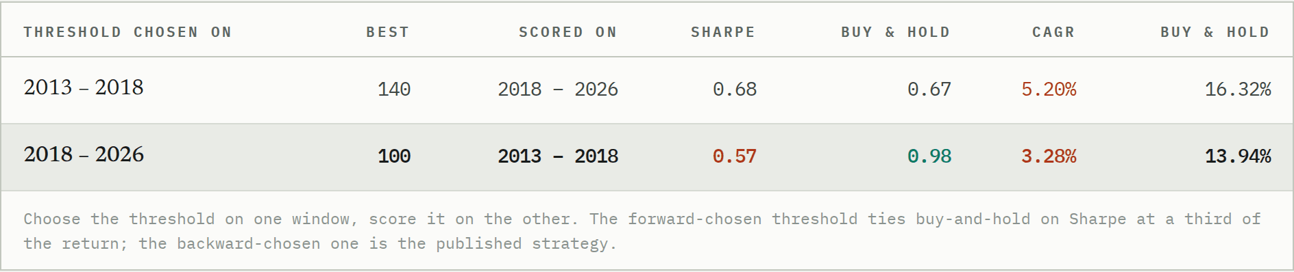
Then the walk-forward, which is the only fair way to choose a parameter. Pick the threshold on 2013 to 2018 without looking at what came after and you pick 140. Run 140 on 2018 to 2026 and you get a Sharpe of 0.68 against buy-and-hold's 0.67, at a third of the return (5.2% a year against 16.3%), on 133 trades in eight years. Pick on 2018 to 2026 and you pick 100, which then loses 0.57 to 0.98. Neither direction beats the index.
Trades entered between 100 and 110 on the oscillator earned $540 each in the window the threshold was chosen in, and $1 each outside it.
Regime is real, and we are not withdrawing section 03. At every threshold the average trade is larger after 2018 — two to three times larger across the readable range — and about 1.5× of that is simply the volatility difference between the two periods (21.7% against 14.0%). But regime lifts the whole family a little. It does not explain why one threshold, the one we chose, beats the thresholds twenty points either side of it by a quarter to half a Sharpe point in the window we chose it in. A year-block bootstrap puts the gap between 100 and its immediate neighbours inside noise, which is the point: the hump is real, its height at 100 is inflated by selection, and the whole hump is absent out of sample.
So the verdict changes. Not "unproven". The strategy does not beat holding the index on any threshold it did not get to choose after the fact. The paper lane keeps running at 100, because re-tuning it on this test would be the exact sin the test describes, and its job was never validation. And the parameter neighbourhood in both windows becomes a standard gate here, applied to everyone we examine, before any in-versus-out-of-sample claim is published.
04 / THE ARITHMETIC OF WAITING
What six months of live trading can and cannot prove
The obvious answer is to run it forward and find out. We looked at what that would actually deliver, and the answer is sobering.
The signal fires on 22% of sessions — about 69 trades a year, a median of five a month, and across 164 months of history there has never been a month with zero trades. So the lane is healthy; a couple of quiet sessions means nothing. A six-month run contains a median of 31 trades, ranging from 20 in the quietest stretch to 94 in the busiest.
Now the problem. Thirty-one trades at a 55% win rate has a standard deviation of 2.8 wins. Two standard deviations either side puts the observed win rate anywhere between 37% and 73% on luck alone. A six-month paper run cannot distinguish a working strategy from a broken one. It cannot even distinguish either from a coin.
So we are changing what we claim the lane is for. It is not validating the edge, because it mathematically cannot. It is proving the machinery — that orders fill where the backtest says they fill, that the entry window is respected, that positions flatten — and it is accumulating forward out-of-sample evidence that will be worth something in three years and nothing in six months. We will keep running it, and we will stop describing it as a test.
05 / THE TRANSFERABLE PART
The test you should run on us
Three questions, and they are the ones we now apply to everything including ourselves.
Where does the sample end and the tuning begin? Almost every published strategy has a window in which it was developed. Ask which one it is, then ask to see the result outside it. If the author cannot tell you where that boundary sits, the whole result is in sample.
What did the benchmark do in each half? A strategy that beats a 0.67-Sharpe market and loses to a 0.95-Sharpe market has told you something about itself, but not what the headline says. Compare within each regime, not across the average.
How many trades would it take to know? Run the arithmetic before you run the strategy. If the sample you are going to collect cannot separate the hypotheses, waiting is not evidence-gathering, it is just waiting.
We are not retiring this strategy. It has a real and statistically strong result in one half of its history, a weak but positive one in the other, and a defensive profile that is genuinely useful. What it does not have is proof that it beats holding the index, and we are not going to write that it does. The addendum sharpens this: the strong half is the half the threshold was chosen in, and no threshold beats the index in the other.
Method
Data: Dukascopy 1-minute bid, resampled to 10-minute bars, gap-repaired to zero missing weekdays. 4,253 sessions, 2 January 2013 to 21 August 2026. Signal computed on bar close, filled at the next bar's open, flat at 16:00 New York. Friction one index point per round trip.
Account construction: each trade expressed as a percent of the notional it controlled at entry (index level × $20 per Nasdaq point), compounded daily, with idle capital earning the one-month Treasury bill rate from the Ken French data library. Benchmark is the total return of holding the index over the identical sessions.
On leverage: the 3× rows are priced without a borrowing charge, which is defensible only because this strategy is flat by the close every day — there is no overnight financing, and futures embed the risk-free rate in the basis. A cash-equity strategy carrying positions overnight would need the real margin rate charged against it, and when we did that to Connors RSI(2) it destroyed the edge. Worst single day at 1× is −5.45% of notional, so −16.4% at 3×.
Addendum: eleven thresholds, 50 to 150 in steps of ten, each window run on its own with the first 200 bars skipped, fixed calendar windows 2013-01-01 to 2018-12-01 and 2018-12-01 to 2026-09-01. At 100 the trade lists are identical to those behind sections 01 and 02. Walk-forward chooses the threshold by Sharpe on one window and scores it on the other. Bootstrap: 4,000 resamples of calendar years.
Backtested results are hypothetical and do not represent returns any investor achieved. This is research, not investment advice.